
Image Display
The most basic processing step after image calibration is simply altering the way in which the image is displayed so it looks best on your computer screen. Computer screens are limited to displaying 256 shades of grey. This is all that is necessary to produce images which look pleasing to the human eye. The number of shades that a monitor or CCD camera can display is known as bit depth. A bit is an exponential unit, described by a simple equation stating that an n-bit system can display 2n shades. Thus, a computer monitor is an 8-bit system since 28 = 256. The problem of displaying a CCD image arises from the fact that most CCD cameras are 16-bit systems. Since bits are exponential, the numbers get real big real quick: 216 = 65,536!
Note: Not all cameras are 16-bit systems. Some are 14-bit or 12-bit. But even a 12-bit system has 4096 levels of grey, still much more than an 8-bit monitor.
How do you get 65,536 shades of grey into the 256 shades a computer monitor can display? By scaling the image.
Scaling
Image processing software automatically scales a CCD image to display it within the limits of the 8-bit computer monitor. However, this automatic scaling rarely produces the best-looking image. Usually, when an image is first opened in a program the background is too bright and the highlights are washed out. This will, of course, depend on many factors including the type of object imaged.
We start by opening an image, in this case the Swan Nebula, M17. You can see that the background is not displayed as black but rather grey. The bright core of the nebula is washed out.

Each software package has a different way of changing the display values. In MaxIm DL this is the Screen Stretch function (but most programs work in a similar fashion). The screen stretch displays the image histogram, which is a graph of pixel brightness vs. number of pixels. For our raw image above the Screen Stretch window looks like this:

The red triangle of the left side of the image determines the black point of the image. Everything left of the red triangle is displayed as pure black. The green triangle sets the white point. Everything right of the green triangle is displayed as pure white. The values between the red and green triangles are the Range that is displayed on the screen. The current black point is 0 and the current white point is 3735. This means the Range is 3735. This is the range of values that will be compressed into 256 values to be displayed on the screen.
Since the background is not displayed as black, we know that the darkest pixels values in the image must be higher than 0. This is due to sky background glow from light pollution, among other factors. To make the background black, without losing any faint detail, bring the red slider up to the toe (left end) of the histogram.

Now the Screen Stretch window shows that the black value was increased to 573. The white point has not been adjusted yet. The background is now displayed as black, and the Range has been decreased to 3162.

Now, what about the washed out details in the bright parts of the image? They imply that the brightest parts of the image have pixel values above 3735. To bring them back into view on the screen, the white point slider (green triangle) must be moved to the right. This increases the Range and brings more pixel values into view.

In this case the white point was increased to 9670. Now, only pixels higher in value than 9670 are displayed as white. The Range is now 9097.

So why not move the white point slider all the way up to 65,535, which would include all the remaining shades of grey in the original 16-bit image? Because the entire range has to be divided up into 256 values (or technically 254, since pure black and pure white take up the 0 and 255 values). One look at the histogram shows that most of the pixels in this image (and almost any astronomical image) are crowded toward the black end of the graph. In other words, most of the values are very dark. Not only is the sky dark, but also the main parts of the nebula itself are faint and yields dim pixel values. Only the few bright areas of the nebula and a couple bright stars contribute to high pixel values.
So, if a wide range of pixel values is displayed, evenly divided into the available 254 shades of grey, most of the "important" pixels (the ones that make up the bulk of the object we're imaging) will be displayed over a small range of dark shades of grey. The result is the image above, where the bright portions of the nebula are visible, but at the expense of making the faint parts invisible or extremely faint.
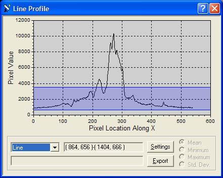
Check out the Line Profile below. This shows the pixel values through a section of the M17 image, including the brightest part of the nebula. The peak pixel values are around 10,000, with the most of the nebulosity and background in the range of 500 to 2000.

Above: A profile of the pixel values in the Swan Nebula image. These values are along a line through the central part of the nebula. The bright parts of the nebula have values around 10,000. Most of the lower pixel values (under 2000) are the faint parts of the nebula.
When the Range is set as shown in the second M17 image, every pixel with a value higher than 3735 is white. This places the values in the brightest areas of the nebula well above pure white. In the profile shown below everything within the blue box is displayed in the image (with the black point set at 573 and the white point at 3735). Every value above the top blue line is white, everything below is black. (Note that the background sky is not captured in this profile and so all the black pixels actually fall outside the area shown).

If the Range is increased so that only pixels of value 9790 and above are white, then the pixels around 2000 (in the faint parts of the nebula) are closer to the black end of the brightness scale. They appear much dimmer. It is best to choose a Range value which is high enough to bring out as much detail as possible in the middle to brighter areas but is still low enough to make these areas bright enough to easily see.
The display compresses the selected values evenly into 256 levels. Examine the profile below. Dividing the full range of brightness evenly puts the brightest values into about 75% of the brightness levels. Only the remaining 25% are left for the faint parts of the nebula. By lowering the Range the detailed arms take up a greater portion of the brightness levels, meaning they can be better displayed. However, this is done at a loss of detail in the highlights.

Above: When the white point setting is moved to 9790, most of the pixels fall into the Range. However, most of the range is taken up by the few bright pixels, while the majority of pixels (the faint ones) are displayed in only 25% of the range, making them difficult to discern.
So far the Range has been divided evenly into the 256 display levels. Is it possible to divide them in another fashion so that both bright and dim portions of an image can be displayed at the same time? Fortunately the answer is Yes! However, we have so far been dealing only with display scaling and not rescaling image data which affects the actual information in the image. This is the next step!
Log Scaling
The most common method employed to rescale the actual image data itself is called Log Scaling. Instead of a linear method of scaling, Log Scaling uses a logarithmic function to display the image. Bright and faint details are scaled differently so that both can be seen at the same time. This function works especially well on high-contrast objects such as spiral galaxies and certain bright nebulae such as the Great Orion Nebula and, of course, the Swan Nebula, as seen here.

Above: This image shows the effects of log scaling. Compare to the last M17 image above to see that both bright and faint details can be more easily seen.

Log scaling works by compressing the data into a smaller range. Instead of the bright pixels taking up 75% of the range, they now only comprise only about 50% of the range while the faint pixels have been expanded to take up the remaining 50%. Now both bright and faint details can be seen in the same image.

Above: Line profile after log scaling. Note that the range of values follow a more linear curve, rather than the sharply spiked profile seen before. Also, the scale has changed, increasing the overall pixel values, but the important thing to note is that the curve is compressed relative to the previous ones.
Other forms of scaling are available, but these functions should suffice for now. Once you have mastered these techniques, check out theAdvanced Image Processing section for more ways to scale your CCD images.
Note: Remember that Log Scaling permanently affects the data in the image, whereas the previous scaling examples dealt only with how the image was displayed.

Above: The final color image of the Swan Nebula. This image was taken using narrowband filters, but the techniques explained here are the same for any type of imaging.